# 1) load data
# from {SLmetrics}
data("wine_quality", package = "SLmetrics")Using {lightgbm} and {SLmetrics} in classification tasks
In this section a gradient boosting machine (GBM) is trained on the wine quality-dataset, and evaluated using {SLmetrics}. The gbm trained here is a light gradient boosting machine from {lightgbm}.1
Data preparation
# 1.1) define the features
# and outcomes
outcome  <- wine_quality$target$class
features <- wine_quality$features

# 2) split data in training
# and test

# 2.1) set seed for
# for reproducibility
set.seed(1903)

# 2.2) exttract
# indices with a simple
# 80/20 split
index <- sample(1:nrow(features), size = 0.95 * nrow(features))

# 1.1) extract training
# data and construct
# as lgb.Dataset
train <- features[index,]
dtrain <- lightgbm::lgb.Dataset(
    data  = data.matrix(train),
    label = as.numeric(outcome[index]) - 1
)
# 1.2) extract test
# data
test <- features[-index,]


# 1.2.1) extract actual
# values and constuct
# as.factor for {SLmetrics}
# methods
actual <- as.factor(
    outcome[-index]
)

# 1.2.2) construct as data.matrix
# for predict method
test <- data.matrix(
    test
)
Training the GBM
The GBM will be trained with default parameters, except for the objective, num_class and eval.
# 1) define parameters
training_parameters <- list(
    objective     = "multiclass",
    num_class     = length(unique(outcome))
)
Evaluation function
# 1) define the custom
# evaluation metric
eval_fbeta <- function(
    dtrain,
    preds) {

        # 1) extract values
        actual    <- as.factor(dtrain)
        predicted <- lightgbm::get_field(preds, "label")
        value     <- fbeta(
            actual    = actual,
            predicted = predicted,
            beta      = 2,
            # Use micro-averaging to account
            # for class imbalances
            micro     = TRUE
        )

        # 2) construnct output
        # list
        list(
            name          = "fbeta",
            value         = value,
            higher_better = TRUE
        )

}
Training the GBM
model <- lightgbm::lgb.train(
    params  = training_parameters,
    data    = dtrain,
    nrounds = 100L,
    eval    = eval_fbeta,
    verbose = -1
)
Evaluation
The predicted classes can be extracted using predict() - these values will be converted to factor values
# 1) prediction
# from the model
predicted <- as.factor(
    predict(
        model,
        newdata = test,
        type    = "class"
    )
)
Safe conversion
predicted <- factor(
predict(
model,
newdata = test,
type = "class"
),
labels = levels(outcome),
levels = seq_along(levels(outcome)) - 1
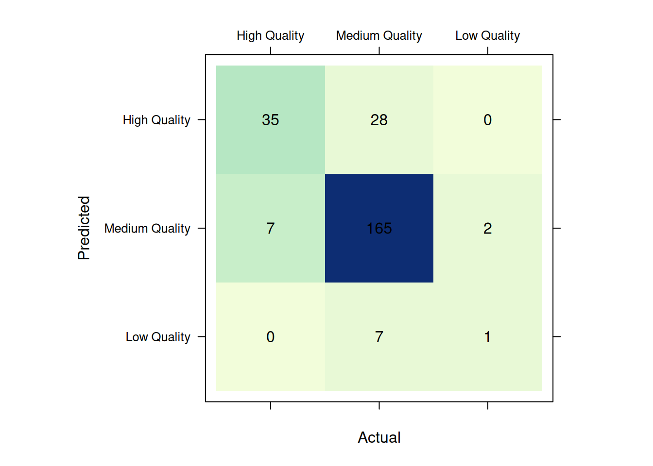
)# 1) construct confusion
# matrix
confusion_matrix <- cmatrix(
actual = actual,
predicted = predicted
)
# 2) visualize
plot(
confusion_matrix
)
# 3) summarize
summary(
    confusion_matrix
)
#> Confusion Matrix (3 x 3)
#> ================================================================================
#> High Quality Medium Quality Low Quality
#> High Quality 35 28 0
#> Medium Quality 7 165 2
#> Low Quality 0 7 1
#> ================================================================================
#> Overall Statistics (micro average)
#> - Accuracy: 0.82
#> - Balanced Accuracy: 0.54
#> - Sensitivity: 0.82
#> - Specificity: 0.91
#> - Precision: 0.82Receiver Operator Characteristics
# 1) prediction
# from the model
response <- predict(
        model,
        newdata = test
    )
The response can be passed into the ROC()-function,
# 1) calculate the reciever
# operator characteristics
roc <- ROC(
    actual   = actual,
    response = response
)

# 2) print the roc
# object
print(roc)
#> threshold level label tpr fpr
#> 1 Inf 1 High Quality 0.0000 0
#> 2 0.973 1 High Quality 0.0159 0
#> 3 0.973 1 High Quality 0.0317 0
#> 4 0.965 1 High Quality 0.0476 0
#> 5 0.957 1 High Quality 0.0635 0
#> 6 0.949 1 High Quality 0.0794 0
#> 7 0.931 1 High Quality 0.0952 0
#> 8 0.926 1 High Quality 0.1111 0
#> 9 0.896 1 High Quality 0.1270 0
#> 10 0.896 1 High Quality 0.1429 0
#> [ reached 'max' / getOption("max.print") -- omitted 728 rows ]The ROC()-function returns a data.frame-object, with 738 rows corresponding to the length of response multiplied with number of classes in the data. The roc-object can be plotted as follows,
# 1) plot roc
# object
plot(roc)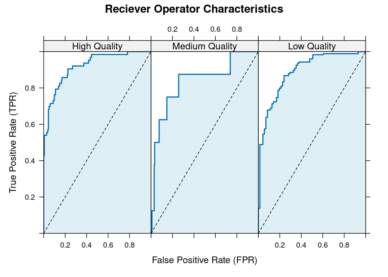
roc.auc(
    actual,
    response
)
#> High Quality Medium Quality Low Quality
#> 0.9200244 0.8888619 0.8349156